Tutorial – tuning a quarter car

A quarter car crosses a bump. We look at the model, tune the damper with a slider, compare runs, let FreeDyn simulate seven dampers at once, and read the trade-off between comfort and road holding off a key figure plot – then check it against the eigenvalues. About 20 minutes.

freedyn2 examples quarter_car     # copies quarter_car.yaml into the current directory
freedyn2 view quarter_car.yaml

1. The model

Open quarter_car.yaml in an editor next to the viewer. It has two bodies – a quarter of the car body (400 kg) and the wheel (40 kg) – each moving only vertically:

parameters:
  m_body: 400.0      # [kg] a quarter of the car
  m_wheel: 40.0      # [kg] wheel, hub, brake, half the link masses
  k_spring: 25000.0  # [N/m] suspension spring
  c_damper: 1800.0   # [N s/m] suspension damper
  k_tire: 200000.0   # [N/m] tire, vertical
  ...
bodies:
  body:
    mass: =m_body                   # a formula of the parameters
    ...
joints:
  body_guide: {type: prismatic, body1: body, location: [0, 0, 0.65]}       # vertical only
  wheel_guide: {type: prismatic, body1: wheel, body2: body, location: [0, 0, 0.3]}
forces:
  suspension:
    type: spring_damper
    body1: wheel
    body2: body
    stiffness: =k_spring
    damping: =c_damper
    preload: =-m_body * 9.81        # compression carries the body
  tire:
    type: expression_force          # a force law you write yourself
    body1: wheel
    direction: [0, 0, 1]
    force: >-
      (m_body + m_wheel) * 9.81
      + k_tire * (if_else((t > t0) * (t < t0 + L / v), 0.5 * h * (1 - cos(2 * pi * v * (t - t0) / L)), 0) - z_wheel)
      - c_tire * vz_wheel

• parameters are named numbers. Any number in the model can be a formula of them, written with = as in a spreadsheet. The viewer turns every parameter into a slider.
• The prismatic joints leave each body one direction to move in: the joint's z axis, vertical by default.
• The tire is an expression force: the static load, plus the tire spring compressed by the road height under the wheel minus the wheel's travel z_wheel. The road is a cosine bump of height h and length L, crossed at speed v from t0 on. z_wheel and vz_wheel are measures defined at the end of the file.

The Checks panel says 2 bodies · 2 joints · 2 forces · 2 DOF · 440 kg and no findings; the total mass is also checked against the reference in the file's checks section.

2. Look at the results

Press space to play. Then plot, by clicking in the channel list on the right:

• body.R_z – the height of the car body,
• tire.value – the vertical tire force (the wheel load),
• body.Rddot_z – the vertical acceleration of the body, our comfort measure. It is the acceleration the solver computes, not a difference quotient of the velocity.

With ƒ formula you add channels that are not in the results, e.g. the suspension travel travel = body.R_z - wheel.R_z.

Drag a range in a plot to zoom to the bump (0.4 to 2 s); all time plots follow.

3. Tune the damper

Open Tune on the right. Every parameter has a slider. Set c_damper to 800 and watch the header:

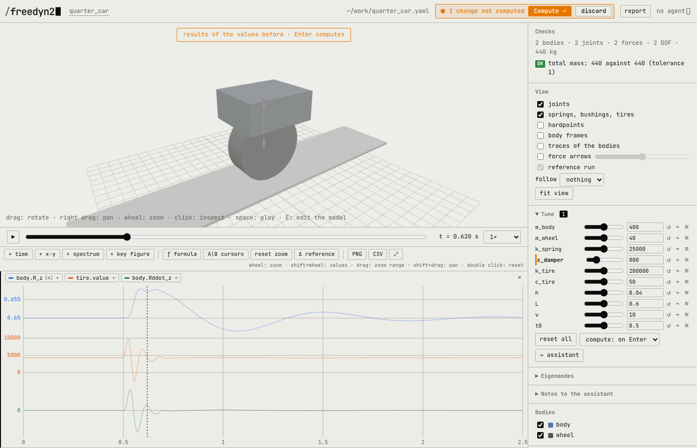
• The header turns amber: 1 change not computed. The 3D view and the curves fade – they still show the results of the old values.
• With the default policy adaptive, a model this fast (a quarter of a second) is computed right away; a slower one waits for Compute ⏎ or Enter. While it computes, the header is blue and the new curves grow over the faded ones.
• When it is done the header is green again: up to date.

The model file has not changed. Tuned values live in the viewer until you take them over (step 8).

4. Compare runs

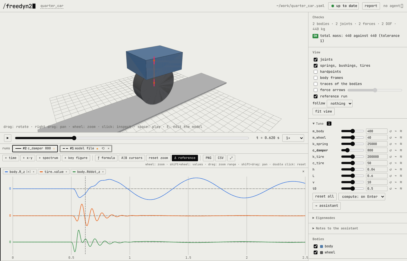
Every simulation is a run in the strip above the plots: #1 model file, #2 c_damper 800. Click ☆ on #1 to make it the reference: its curves are dashed in every plot, its bodies grey in the 3D view. Then press Δ reference: the plots show each run minus the reference – small differences that hide in an overlay become obvious.

5. A fan of variants

Instead of trying one damper after another, press ≋ next to the c_damper slider: seven values over the slider's range are simulated at once, in parallel. The time plots show them as a fan, blue for the softest, red for the hardest. A key figure plot appears below: choose peak-peak – it is taken over the visible time range, so zoom to the bump first.

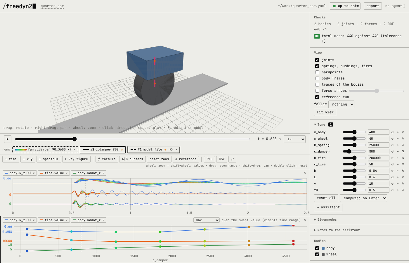
The two key figures pull in opposite directions:

c_damper [N s/m]	90	675	1260	1845	2430	3015	3600
body acceleration body.Rddot_z, peak-peak [m/s²]	7.0	10.4	13.9	16.5	18.2	19.3	20.2
tire force tire.value, peak-peak [kN]	19.7	14.7	12.8	12.3	11.8	11.5	11.3

(over 0.4 to 2 s; the slider's range is 0 to twice the file's value, the fan starts a little above 0)

A soft damper is comfortable (small body acceleration) but lets the wheel load swing – less grip on a bumpy road; a hard one keeps the wheel on the road and shakes the passengers. The key figure plot shows where the knee is.

6. Why: the eigenvalues

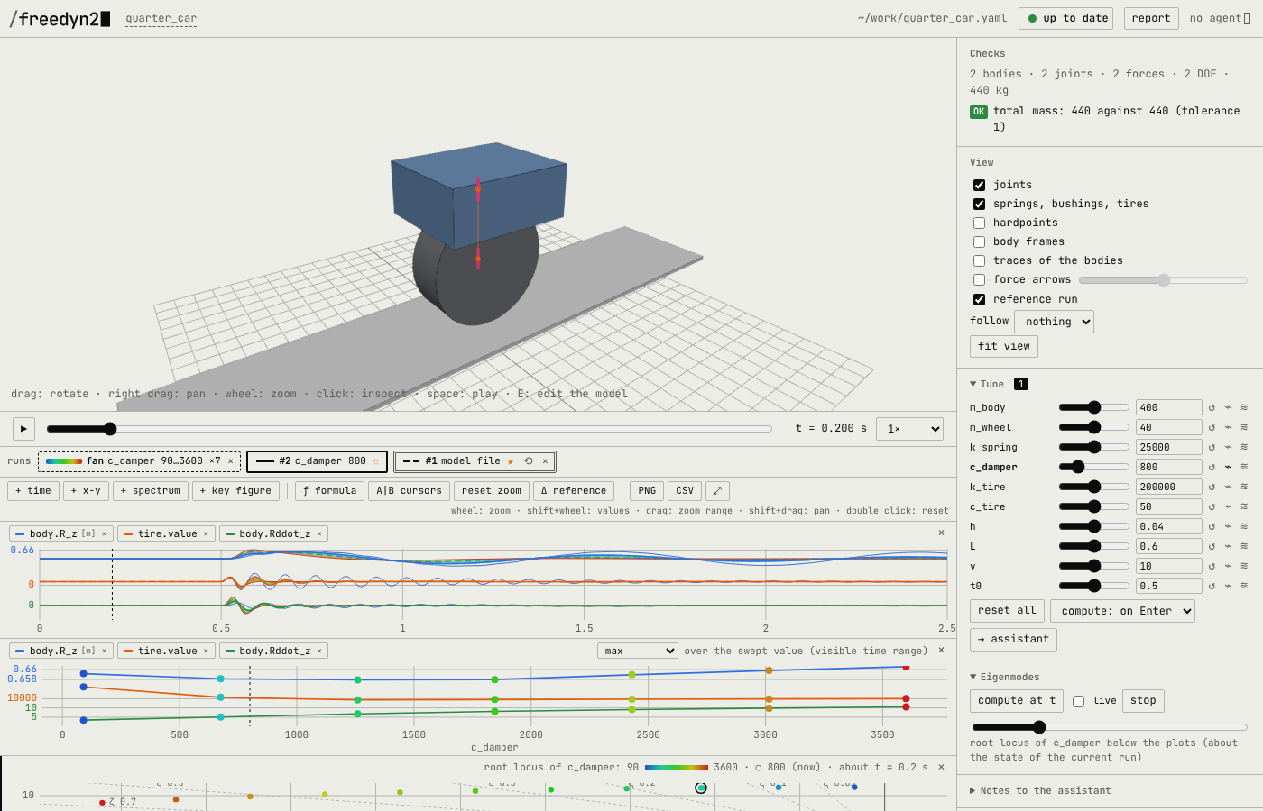
Open Eigenmodes and press compute at t (at a time before the bump, when the car is at rest). Two modes:

• body bounce at 1.17 Hz, damping ratio 24 %,
• wheel hop at 11.2 Hz, damping ratio 32 %.

Click one to see it move. Now tick live and move the c_damper slider: the frequencies and damping ratios follow at once, before anything is simulated (▲▼ shows the change). At 500 N s/m both modes are barely damped (7 % and 9 %); at 5000 the body mode is critically damped – the car no longer bounces, it is held. Press ⌁ next to the slider for the whole picture, the root locus: each eigenvalue for eleven damper values, coloured from soft to hard, with lines of equal damping ratio.

7. Notes to the assistant

If an assistant works on this model with you (Working with an assistant), open Notes to the assistant and write what you found, e.g. "c_damper 2400 is the best compromise, take it into the model". The note carries the time, the selected element, the plotted channels, the tuned values and a picture of the view; the assistant reads it, changes the file and answers – the answer appears under the note.

8. Keep the result

Tuned values are not written into the model file by the viewer – the file stays yours (or your assistant's). Either type the value into the file (the viewer reloads and shows the run as file v2), or send it with → assistant. Report writes one HTML file with the view, the plots, the checks, the tuned values and the eigenmodes, to print or pass on.

What next

• Change the model: give the body pitch by adding a second wheel, or replace the expression tire by the tire element on a road.
• Read the viewer page for the plots (x-y, spectrum, cursors, formulas).
• Let an assistant run a sweep over two parameters and report the best pair.